Figure 5.1: Noise characteristics
In this chapter, we will explain the noise used in computer graphics. Noise was developed in the 1980s as a new method of image generation for texture mapping. Texture mapping, which attaches an image to an object to create its complexity, is a well-known technique in today's CG, but computers at that time had very limited storage space. Using image data for texture mapping was not compatible with the hardware. Therefore, a method for procedurally generating this noise pattern was devised. Naturally occurring substances and phenomena such as mountains, desert-like terrain, clouds, water surfaces, flames, marble, grain, rocks, crystals, and foam films have visual complexity and regular patterns. .. Noise can generate the best texture patterns for expressing such naturally occurring substances and phenomena, and has become an indispensable technique when procedurally wanting to generate graphics. Typical noise algorithms are Ken Perlin 's achievements, Perlin Noise and Simplex Noise . Here, as a stepping stone to many applications of noise, I would like to explain mainly the algorithms of these noises and the implementation by shaders.
The sample data in this chapter is from the Common Unity Sample Project.
Assets/TheStudyOfProceduralNoise
It is in. Please also refer to it.
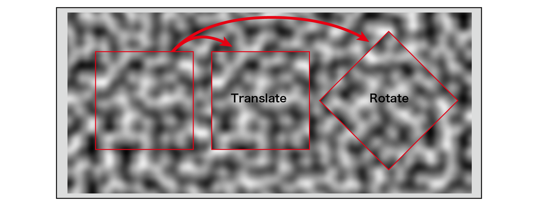
The word noise means a noisy sound that can be translated as noise in the field of audio, and also in the field of video, it usually refers to general unnecessary information for the content to be processed or to show image roughness. Also used. Noise in computer graphics is a function that takes an N-dimensional vector as an input and returns a scalar value (one-dimensional value) of a random pattern with the following characteristics.
Figure 5.1: Noise characteristics
Noise can be used for the following purposes by receiving an N-dimensional vector as an input.
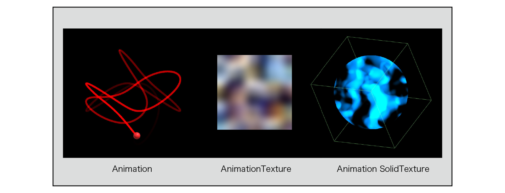
Figure 5.2: Noise application
We will explain the algorithms for Value Noise , Perlin Noise , Improved Perlin Noise , and Simplex Noise .
Although it does not strictly meet the conditions and accuracy of a noise function, we will introduce a noise algorithm called Value Noise , which is the easiest to implement and helps you understand noise.
For two dimensions, define an evenly spaced grid on each of the x and y axes. The grid has a square shape, and at each of these grid points, the value of the pseudo-random number is calculated with reference to the coordinate values of the grid points. In the case of 3D, a grid is defined at equal intervals on each of the x, y, and z axes, and the shape of the grid is a cube.
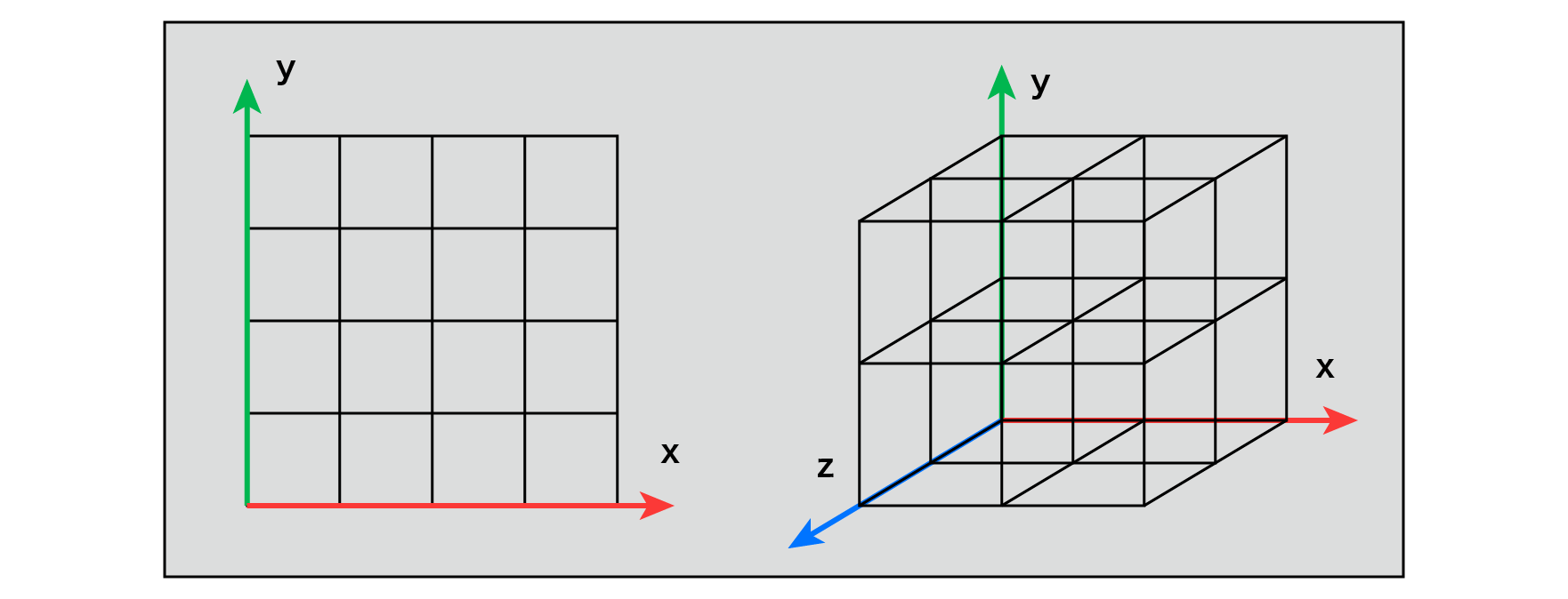
Figure 5.3: Lattice (2D), Lattice (3D)
A random number is a sequence of numbers that are randomly arranged so that they have the same probability of appearing. There are also random numbers called true random numbers and pseudo-random numbers. For example, when rolling a dice, it is impossible to predict the next roll from the previous roll, and such a random number is a true random number. Is called. On the other hand, those with regularity and reproducibility are called pseudo-random numbers (Pseudo Random) . (When a computer generates a random number sequence, it is calculated by a deterministic calculation, so most of the generated random numbers can be said to be pseudo-random numbers.) When calculating noise, the same result can be obtained by using common parameters. Use the pseudo-random number that gives.

Figure 5.4: Pseudo-random numbers
By giving the coordinate values of each grid point to the argument of the function that generates this pseudo-random number, the value of the pseudo-random number unique to each grid point can be obtained.
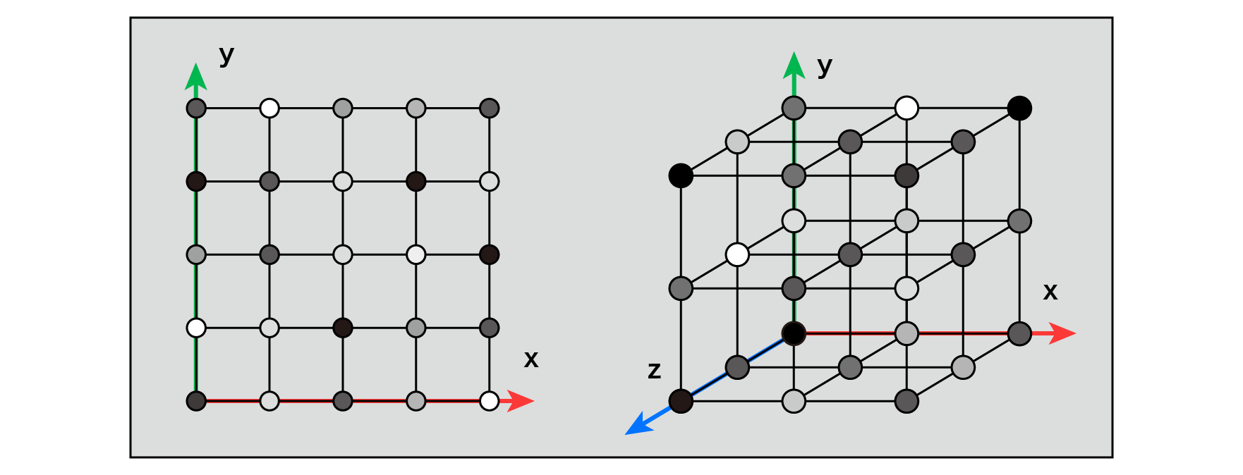
Figure 5.5: Pseudo-random numbers on each grid point
There are values A and B, and the value of P between them changes linearly from A to B, and finding that value approximately is called linear interpolation . This is the simplest interpolation method, but if you use it to find the value between the grid points, the change in the value will be sharp at the start and end points of the interpolation (near the grid point).
Therefore, we use a cubic Hermitian curve as the interpolation factor so that the values change smoothly .
f\left( t\right) =3t^{2}-2t^{3}
When this is changed t=0from t=1to, the value will be as shown in the lower right figure.
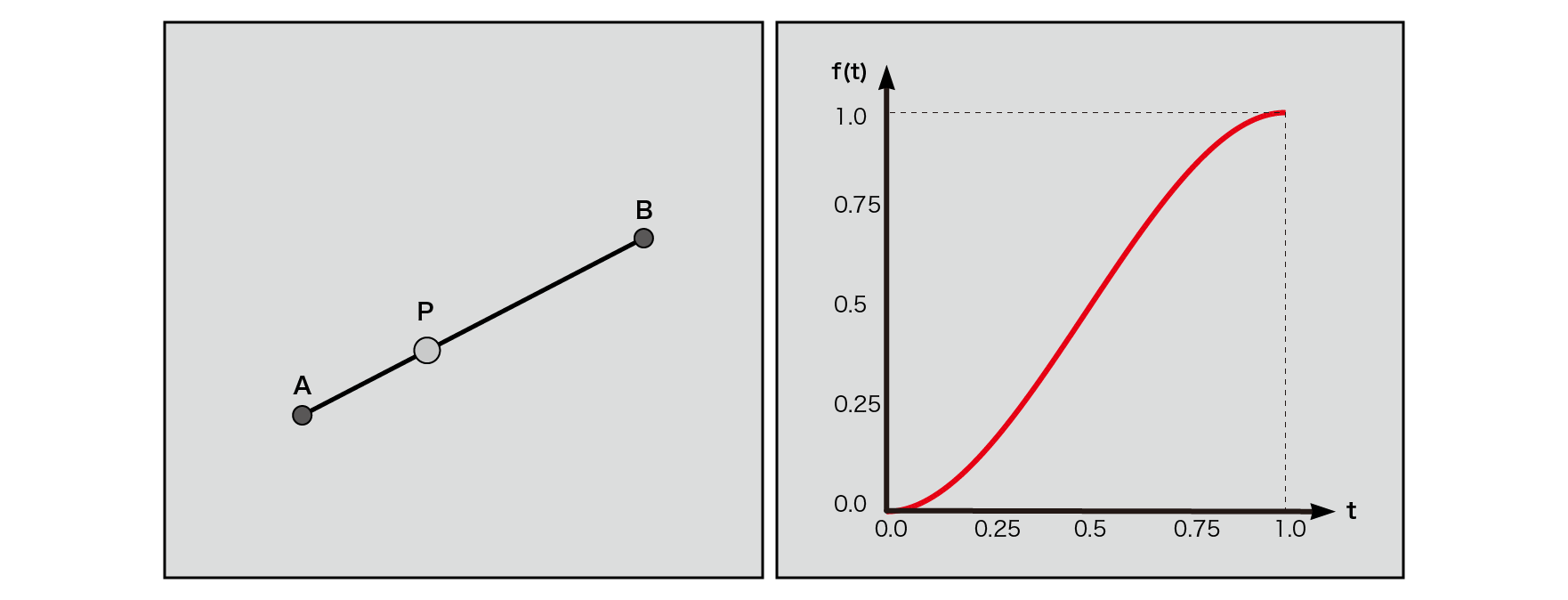
Figure 5.6: Linear interpolation in a two-dimensional plane (left), cubic Hermitian curve
* The cubic Hermitian curve is implemented as a smoothstep function in GLSL and HLSL .
This interpolation function is used to interpolate the values obtained at each grid point on each axis. In the case of 2D, first interpolate for x at both ends of the grid, then interpolate those values for the y-axis, and perform a total of 3 calculations. In the case of 3D, as shown in the figure below, 4 interpolations are performed for the z-axis, 2 for the y-axis, and 1 for the x-axis, for a total of 7 interpolations.
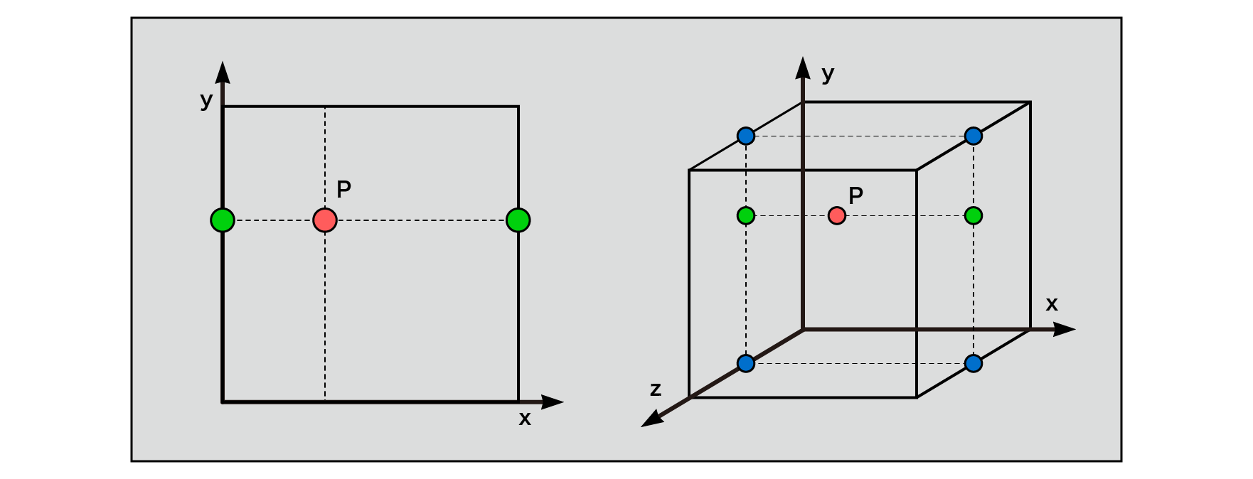
Figure 5.7: Interpolation (2D space), Interpolation (3D space)
I will explain about 2D. Find the coordinates of each grid point.
floor()
The integer part is floor()calculated using a function. floor()Is a function that returns the smallest integer less than or equal to the input real number. When a real number of 1.0 or more is given to the input value, the values 1, 2, 3 ... are obtained and the same values are obtained at equal intervals, so this can be used as the coordinate value of the grid.
Use a frac()function to find the decimal part .
frac()
frac()Returns the decimal value of the given real number and takes a value greater than or equal to 0 and less than 1. This allows you to get the coordinate values inside each grid.
// Coordinate values of grid points float2 i00 = i; float2 i10 = i + float2 (1.0, 0.0); float2 i01 = i + float2(0.0, 1.0); float2 i11 = i + float2 (1.0, 1.0);
If you assign the coordinate values obtained above to the fragment colors R and G, you will get the following image. (For the integer part, since it can take a value of 1 or more, it is scaled so that the result does not exceed 1 for visualization.)
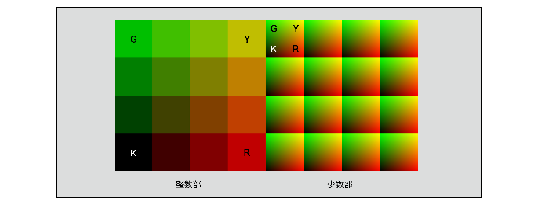
Figure 5.8: Integer and minority parts drawn as RG
Searching the internet for the random function often returns this function as a result.
float rand(float2 co)
{
    return frac(sin(dot(co.xy, float2(12.9898,78.233))) * 43758.5453);
}
Looking at the processing one by one, first, the input two-dimensional vector is rounded to one dimension by the inner product to make it easier to handle, and it is given as an argument of the sin function, multiplied by a large number, and the decimal part is obtained. So, this gives us regular and reproducible, but chaotically continuous values.
The origin of this function is uncertain,
https://stackoverflow.com/questions/12964279/whats-the-origin-of-this-glsl-rand-one-liner
According to the report, it originated from a treatise called "On generating random numbers, with help of y = [(a + x) sin (bx)] mod 1" published in 1998 .
Although it is simple and easy to handle, the cycle in which the same random number sequence appears is short, and if the texture has a large resolution, a pattern that can be visually confirmed occurs, so it is not a very good pseudo-random number.
// Pseudo-random value on the coordinates of the grid points
float n00 = pseudoRandom(i00);
float n10 = pseudoRandom(i10);
float n01 = pseudoRandom(i01);
float n11 = pseudoRandom(i11);
By giving the coordinate value (integer) of each grid point to the argument of the pseudo-random number, the noise value on each grid point is obtained.
// Interpolation function (3rd order Hermitian curve) = smoothstep
float2 interpolate(float2 t)
{
    return t * t * (3.0 - 2.0 * t);
}
// Find the interpolation factor
float2 u = interpolate(f);
// Interpolation of 2D grid
return  lerp(lerp(n00, n10, u.x), lerp(n01, n11, u.x), u.y);
interpolate()Calculate the interpolation factor with a predefined function. By using the decimal part of the grid as an argument, you can obtain a curve that changes smoothly near the start and end points of the grid.
lerp()Is a function that performs linear interpolation and stands for Linear Interpolate . It is possible to calculate the linearly interpolated value of the values given to the first and second arguments, and by substituting u obtained as the interpolation coefficient into the third argument, the values between the grids can be connected smoothly.
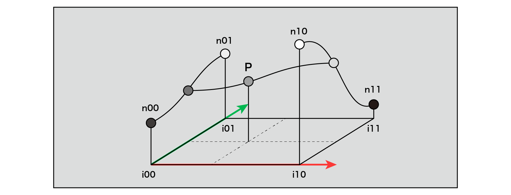
Figure 5.9: Interpolation of grid points (two-dimensional space)
In the sample project
TheStudyOfProceduralNoise/Scenes/ShaderExampleList
When you open the scene, you can see the implementation result of Value Noise . For the code,
There is an implementation in.
Figure 5.10: Value Noise (2D, 3D, 4D) Drawing result
If you look at the result image, you can see that the shape of the grid can be seen to some extent. As you can see, Value Noise is easy to implement, but its isotropic property that its characteristics are invariant when a certain area is rotated is not guaranteed, and it is not enough to be called noise. However, the process of "interpolating the values of pseudo-random numbers obtained from regularly arranged grid points to obtain continuous and smooth values of all points in space" performed in the implementation of Value Noise is , Has the basic algorithmic structure of the noise function.
Perlin Noise is a traditional and representative method of procedural noise and was developed by its name, Ken Perlin . Originally, it was produced in the experiment of texture generation for visual expression of the American science fiction movie "Tron" produced in 1982, which is known as the world's first movie that fully introduced computer graphics, and the result. Was published in a 1985 SIGGRAPH paper entitled "An Image Synthesizer" .
The difference from Value Noise is that the value of the grid point noise is not defined as a one-dimensional value, but as a gradient with a slope (Gradient) . Define a 2D gradient for 2D and a 3D gradient for 3D.
Figure 5.11: Perlin Noise Gradient Vector
Inner product is
\overrightarrow {a}\cdot \overrightarrow {b}=\left| a\right| \left| b\right| \cos \theta
= \left( a.x\ast b.x\right) +\left( a.y\ast b.y\right)
In the vector operation defined in, the geometric meaning is the ratio of how much the two vectors are oriented in the same direction, and the values taken by the inner product are the same direction → 1 , orthogonal → 0 , and vice versa. Orientation → -1 . In other words, finding the inner product of the gradient and the vector from each grid point toward the point P where you want to find the noise value in the grid means that if those vectors point in the same direction, the high noise value will be different. If you are facing the direction, a small value will be returned.
Figure 5.12: Dot Product (Left) Perlin Noise Gradient and Interpolation Vector (Right)
Here, the cubic Hermitian curve is used as a function for interpolation, but Ken Perlin later modified it to a cubic Hermitian curve. We 'll talk about that in the Improved Perlin Noise section.
In the sample project
TheStudyOfProceduralNoise/Scenes/ShaderExampleList
If you open the scene, you can see the implementation result of Perlin Noise . For the code,
There is an implementation in.
I will post the implementation for 2D.
// Original Perlin Noise 2D
float originalPerlinNoise(float2 v)
{
// Coordinates of the integer part of the grid
float2 i = floor (v);
// Coordinates of the decimal part of the grid
float2 f = frac(v);
// Coordinate values of the four corners of the grid
float2 i00 = i;
float2 i10 = i + float2 (1.0, 0.0);
float2 i01 = i + float2(0.0, 1.0);
float2 i11 = i + float2 (1.0, 1.0);
// Vectors from each grid point inside the grid
float2 p00 = f;
float2 p10 = f - float2(1.0, 0.0);
float2 p01 = f - float2(0.0, 1.0);
float2 p11 = f - float2(1.0, 1.0);
// Gradient of each grid point
float2 g00 = pseudoRandom(i00);
float2 g10 = pseudoRandom(i10);
float2 g01 = pseudoRandom(i01);
float2 g11 = pseudoRandom(i11);
// Normalization (set the magnitude of the vector to 1)
g00 = normalize(g00);
g10 = normalize(g10);
g01 = normalize(g01);
g11 = normalize(g11);
// Calculate the noise value at each grid point
float n00 = dot(g00, p00);
float n10 = dot(g10, p10);
float n01 = dot(g01, p01);
float n11 = dot(g11, p11);
// Interpolation
float2 u_xy = interpolate(f.xy);
float2 n_x = lerp(float2(n00, n01), float2(n10, n11), u_xy.x);
float n_xy = lerp(n_x.x, n_x.y, u_xy.y);
return n_xy;
}
There is no unnatural grid shape as seen in Value Noise , and isotropic noise is obtained. Perlin Noise is also called Gradient Noise because it uses a gradient as opposed to Value Noise .
Figure 5.13: Perlin Noise (2D, 3D, 4D) results
Improved Perlin Noise was announced in 2001 by Ken Perlin as an improvement over the shortcomings of Perlin Noise . More details can be found here.
http://mrl.nyu.edu/~perlin/paper445.pdf
Currently, most Perlin Noise is implemented based on this Improved Perlin Noise .
There are two main improvements Ken Perlin has made:
For Hermite curve interpolation, the original of the Perlin Noise in cubic Hermite curve was used. However, if there is in this third-order equation, (when the differential to a result obtained can be further differentiated, that differentiates this) second-order differential 6-12tis t=0, t=1when 0you do not take. Differentiating the curve gives the slope of the tangent. Another derivative gives that curvature, which is non-zero means there is a slight change. As a result, when used as a normal for bump mapping, adjacent grids and values are not exactly continuous, resulting in visual artifacts.
It is a comparison figure.
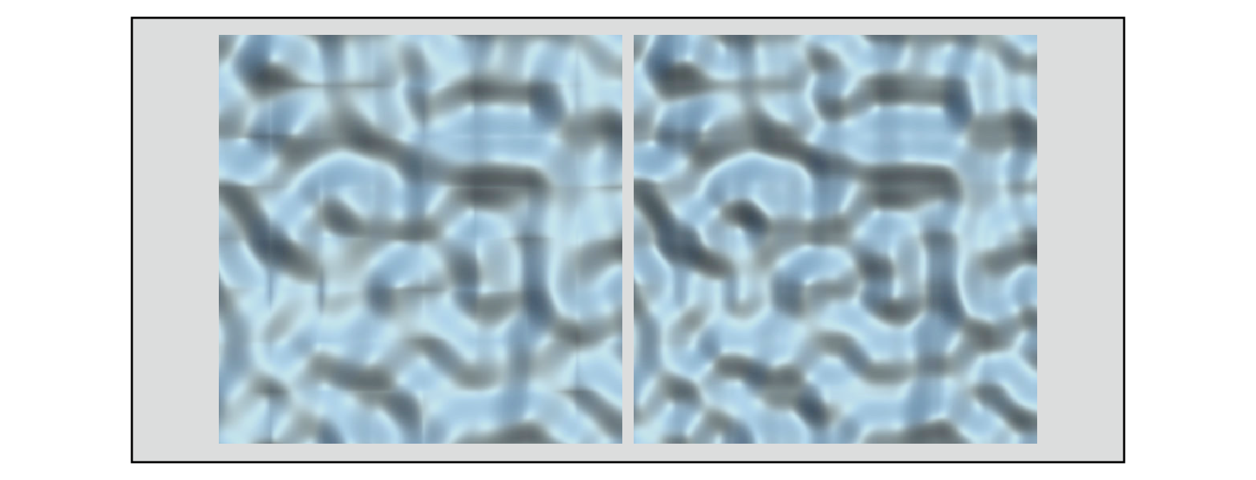
Figure 5.14: Interpolation with a cubic Hermitian curve (left) Interpolation with a fifth-order Hermitian curve (right)
Sample project
TheStudyOfProceduralNoise/Scenes/CompareBumpmap
You can see this by opening the scene.
Looking at the figure, the person who interpolated by the cubic Hermitian curve on the left shows a visually unnatural normal discontinuity at the boundary of the lattice. To avoid this, use the following fifth-order Hermitian curve .
f\left( t\right) =6t^{5}-15t^{4}+10t^{3}
Each curve diagram is shown. ① is a cubic Hermitian curve and ② is a 5th order Hermitian curve .
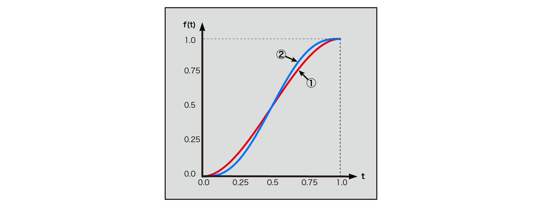
Figure 5.15: 3rd and 5th order Hermitian curves
t=0, t=1You can see that you have a smooth change around. Since both the 1st derivative and the 2nd derivative are at t=0or t=1at times 0, continuity is maintained.
Think about 3D. The gradient G is evenly distributed in a spherical shape, but the cubic lattice is short about its axis, long about its diagonal, and has a directional bias in itself. If the gradient is close to parallel to the axis, aligning it with the ones in close proximity can result in unusually high values in those areas due to the close distance, which can result in a spotty noise distribution. In order to remove this gradient bias, we will limit it to the following 12 vectors, with those parallel to the axes and those on the diagonal removed.
(1,1,0),(-1,1,0),(1,-1,0),(-1,-1,0),
(1,0,1),(-1,0,1),(1,0,-1),(-1,0,-1),
(0,1,1),(0,-1,1),(0,1,-1),(0,-1,-1)
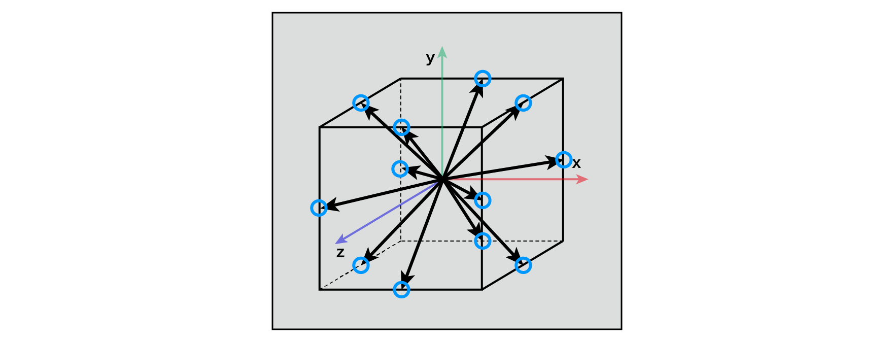
Figure 5.16: Improved Perlin Noise Gradient (3D)
From a cognitive psychological point of view, Ken Perlin states that in reality, the point P in the grid gives enough randomness, and the gradient G does not have to be random in all directions. .. In addition, for example, (1, 1, 0)the (x, y, z)inner product of, simply x + ycan be calculated as, to simplify the inner product calculation to be performed later, you can avoid a lot of multiplication. This removes 24 multiplications from the calculation and keeps the calculation cost down.
In the sample project
TheStudyOfProceduralNoise/Scenes/ShaderExampleList
If you open the scene, you can see the implementation result of Improved Perlin Noise . For the code,
This improved Perlin Noise implementation is based on the one published in the paper "Effecient computational noise in GLSL" , which will also be introduced in the next Simplex Noise . (Here it's called Classic Perlin Noise , so it's a bit confusing, but I'm using that name.) This implementation is different from what Ken Perlin described in the paper for gradient calculations, but it gives quite similar results.
You can check the original implementation of Ken Perlin from the URL below.
http://mrl.nyu.edu/~perlin/noise/
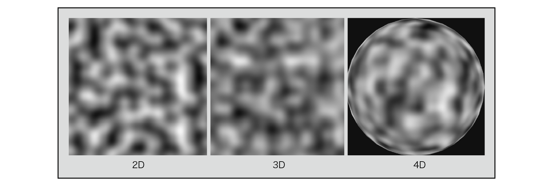
図5.17: Improved Perlin Noise(2D, 3D, 4D)
The figure below compares the noise gradient with the results. The left is the original Perlin Noise and the right is the Improved Perlin Noise .
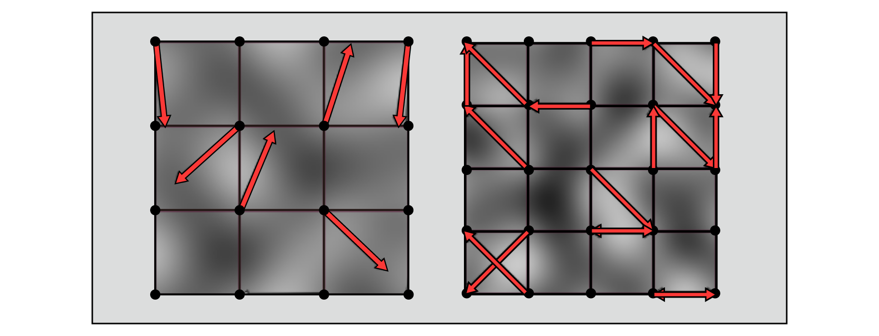
Figure 5.18: Perlin Noise, Improved Perlin Noise Gradients and Results Comparison
Simplex Noise was introduced by Ken Perlin in 2001 as a better algorithm than traditional Perlin Noise .
Simplex Noise has the following advantages over traditional Perlin Noise .
Here, "Simplex Noise Demystify"
http://staffwww.itn.liu.se/~stegu/simplexnoise/simplexnoise.pdf
I will explain based on the contents of.
Simplex is called a simple substance in the topology of mathematics. A simple substance is the smallest unit that makes a figure. A 0-dimensional simplex is a point , a 1-dimensional simplex is a line segment , a 2-dimensional simplex is a triangle , a 3-dimensional simplex is a tetrahedron , and a 4-dimensional simplex is a 5-cell .
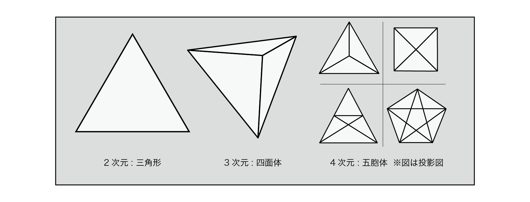
Figure 5.19: Simple substance in each dimension
Perlin Noise used a square grid for 2D and a cubic grid for 3D, but Simplex Noise uses this simple substance for the grid.
In one dimension, the simplest shape that fills the space is evenly spaced lines. In two dimensions, the simplest shape that fills the space is a triangle.
Two of the tiles made up of these triangles can be thought of as crushed squares along their main diagonal.
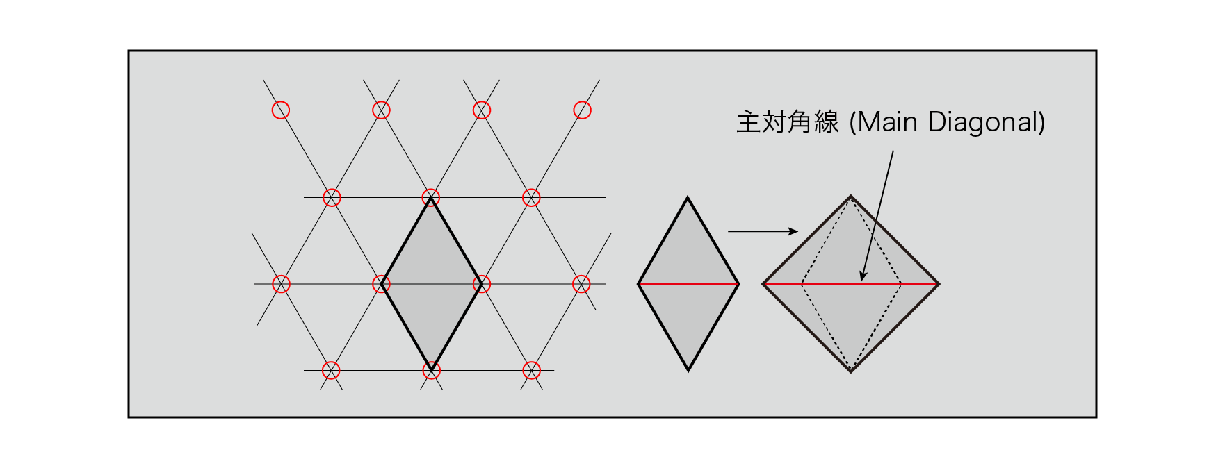
Figure 5.20: Two-dimensional simple substance grid
In three dimensions, the single shape is a slightly distorted tetrahedron. These six tetrahedra form a cube that is crushed along the main diagonal.
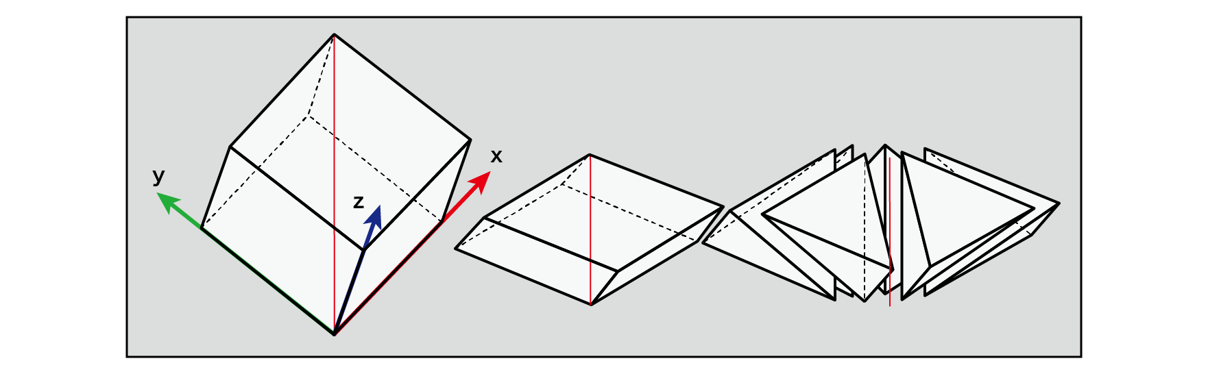
Figure 5.21: Three-dimensional simple substance grid
In 4D, single shapes are very difficult to visualize. Its single shape has five corners, and these 24 shapes form a four-dimensional hypercube that collapses along the main diagonal.
N-dimensional elemental shapes have N + 1 corners, and N! (3! Is 3 × 2 × 1 = 6) shapes fill the N-dimensional hypercube collapsed along the main diagonal. It can be said that.
The advantage of using a simple substance shape for a grid is that you can define a grid with as few angles as possible with respect to the dimension, so when finding the values of points inside the grid, you will interpolate from the values of the surrounding grid points. It is in a place where the number of calculations can be suppressed. The N-dimensional hypercube has 2 ^ {N} corners, while the N-dimensional elemental shape has only N + 1 corners.
When trying to find higher dimensional noise values, traditional Perlin Noise requires O (2 ^ {N}) the complexity of the calculations at each corner of the hypercube and the amount of interpolation for each principal axis . ) It's a problem and quickly becomes awkward. On the other hand, with Simplex Noise , the number of vertices of the simplex shape with respect to the dimension is small, so the amount of calculation is limited to O (N ^ {2}) .
With Perlin Noise, the integer part of the coordinates floor()could be used to calculate which grid the point P you want to find is in. For Simplex Noise, follow the two steps below.
For a visual understanding, let's look at a diagram of the two-dimensional case.
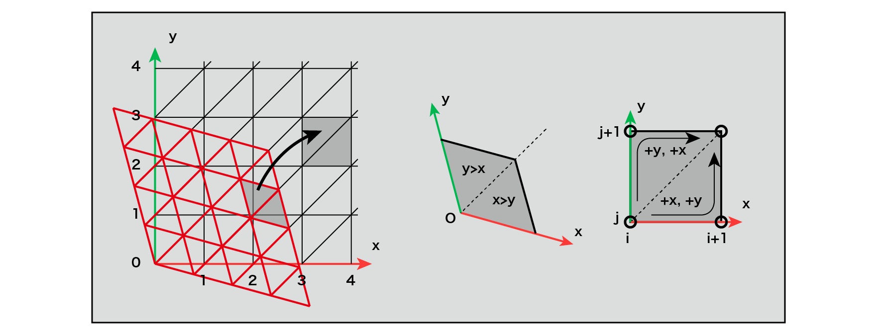
Figure 5.22: Deformation of a single grid in two dimensions
A single grid of two-dimensional triangles can be distorted into a grid of isosceles triangles by scaling. Two isosceles triangles form a quadrangle with one side length (a single unit refers to this quadrangle). (x, y)By looking at the integer part of the coordinates after moving , you can determine which single unit square the point P for which you want to find the noise value is. Also, by comparing the sizes of x and y from the origin of a single unit, it is possible to know which of the units is the single unit including the point P, and the coordinates of the three single points surrounding the point P are determined.
In the case of 3D, the 3D single lattice is regularly arranged by scaling along its main diagonal so that the 2D equilateral triangle single lattice can be transformed into an isosceles triangular lattice. It can be transformed into a cubic grid. As in the case of two dimensions, you can determine which six units belong to a single unit by looking at the integer part of the coordinates of the moved point P. Furthermore, which unit of the unit belongs to can be determined by comparing the relative size of each axis from the origin of the unit.
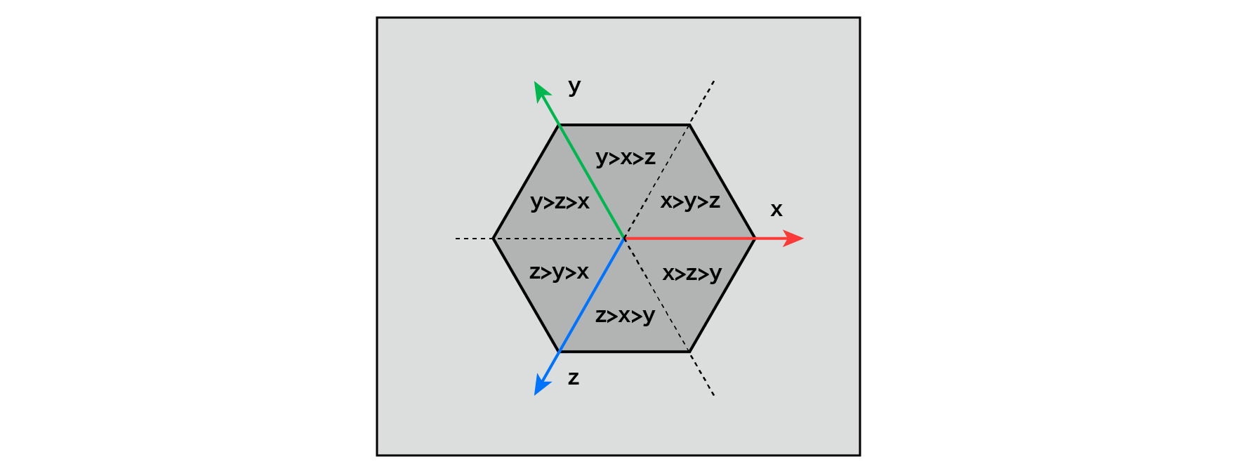
Figure 5.23: Rules for determining which single unit the point P belongs to in the 3D case
The figure above shows a cube formed by a three-dimensional unit along the main diagonal, and belongs to which unit depending on the size of the coordinate values of point P on the x, y, and z axes. It shows the rules of.
In the case of 4D, it is difficult to visualize, but it can be thought of as a rule in 2D and 3D. Coordinates of a four-dimensional hypercube that fills space There are (x, y, z, w)4! = 24 combinations of sizes for each axis, which are unique to each of the 24 units in the hypercube, and the point P belongs to which unit. Can be determined.
The figure below is a two-dimensional single grid visualized in fragment color.
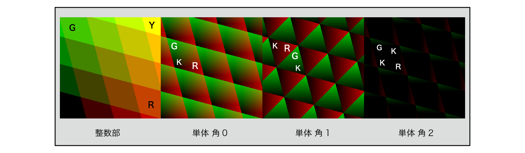
Figure 5.24: Single (2D) integer and minority parts
In conventional Perlin Noise , the values of points inside the grid are calculated from the values of the surrounding grid points by interpolation. However, with Simplex Noise , instead, the degree of influence of the values of the vertices of each simple substance is calculated by a simple sum calculation. Specifically, the extrapolation of the slope of each corner of a single unit and the product of the functions that decay in a radial circle depending on the distance from each vertex are added.
Think about two dimensions.
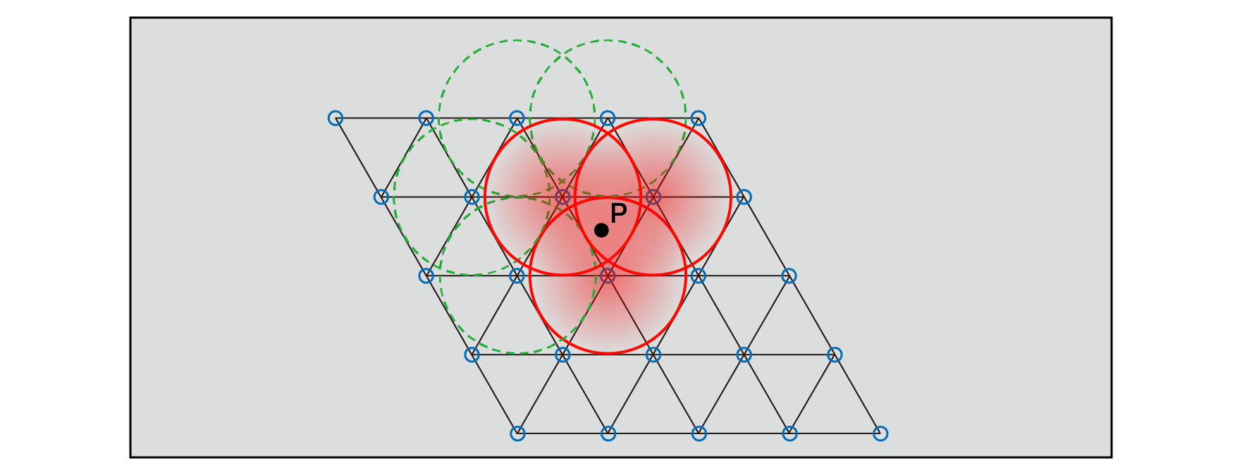
Figure 5.25: Radial circular decay function and its range of influence
The value of the point P inside a single unit only affects the values from each of the three vertices of the single unit that surrounds it. The values of the distant vertices have no effect because they decay to 0 before crossing the single boundary containing the point P. In this way, the noise value at point P can be calculated as the sum of the values of the three vertices and their degree of influence.
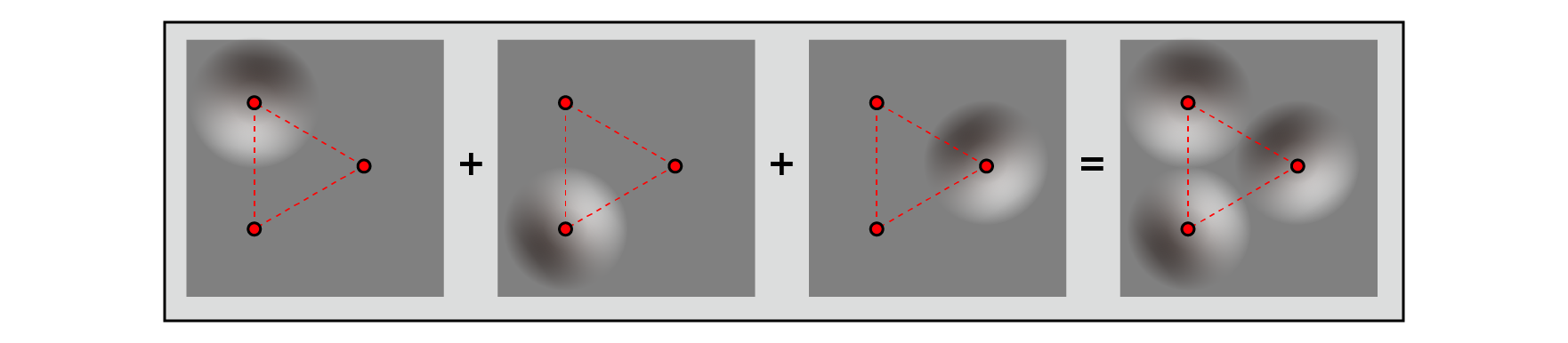
Figure 5.26: Contribution rate and sum of each vertex
The implementation is "Effecient computational noise in GLSL" published by Ian McEwan, David Sheets, Stefan Gustavson and Mark Richardson in 2012.
https://pdfs.semanticscholar.org/8e58/ad9f2cc98d87d978f2bd85713d6c909c8a85.pdf
It is shown in the manner according to.
Currently, if you want to implement noise with a shader, it is an easy-to-use algorithm that is less hardware-dependent, efficient in calculation, and does not require reference to textures. (Probably)
As of April 2018, the source code is managed at https://github.com/stegu/webgl-noise/ . The original was here ( https://github.com/ashima/webgl-noise ), but Ashima Arts, which currently manages it, doesn't seem to be functioning as a company, so it was cloned by Stefan Gustavson.
There are three features of the implementation:
Previously announced noise implementations used tables containing pre-computed index values or bit-swapped hashes for index generation during gradient calculations, but both approaches are shaders. It cannot be said that it is suitable for implementation by. So, for index sorting,
\left( Ax^{2}+Bx\right) mod\ M
We are proposing a method to use a polynomial with a simple form. (Mod = modulo The number of remainders when a certain number is divided (remainder)) For example, \ left (6x ^ {2} + x \ right) mod \ 9 is (0 1 2 3 4 5 6 7 8)for (0 7 8 3 1 2 6 4 5)0 to 8 inputs. Returns 9 unique numbers from 0 to 8.
To generate an index to distribute the gradient well enough, we need to sort at least hundreds of numbers, so we will choose \ left (34x ^ {2} + x \ right) mod \ 289 .
This permutation polynomial is a problem of the precision of variables in the shader language , and truncation occurs when 34x ^ {2} + x> 2 ^ {24} , or | x |> 702 in the integer region . .. So, in order to calculate the polynomial for sorting without the risk of overflow, we do a modulo 289 of x before doing the polynomial calculation to limit x to the range 0-288.
Specifically, it is implemented as follows.
// Find the remainder of 289
float3 mod289(float3 x)
{
    return x - floor(x * (1.0 / 289.0)) * 289.0;
}

// Sort by permutation polynomial
float3 trade-ins (float3 x)
{
    return fmod(((x * 34.0) + 1.0) * x, 289.0);
}
The treatise admits that in 2D and 3D, there is no problem, but in 4D, this polynomial has generated visual artifacts. For 4 dimensions, an index of 289 seems to be inadequate.
Traditional implementations used pseudo-random numbers for gradient calculations, referencing the table containing the indexes and performing bit operations to calculate the pre-calculated gradient indexes. Here, we use a cross-polytope for gradient calculations to get a more efficiently distributed gradient in different dimensions, which is more suitable for shader implementation . A cross-polytope is a generalized shape of a two-dimensional square , a three-dimensional regular octahedron , and a four-dimensional regular six-cell body in each dimension. Each dimension takes a geometric shape as shown in the figure below.
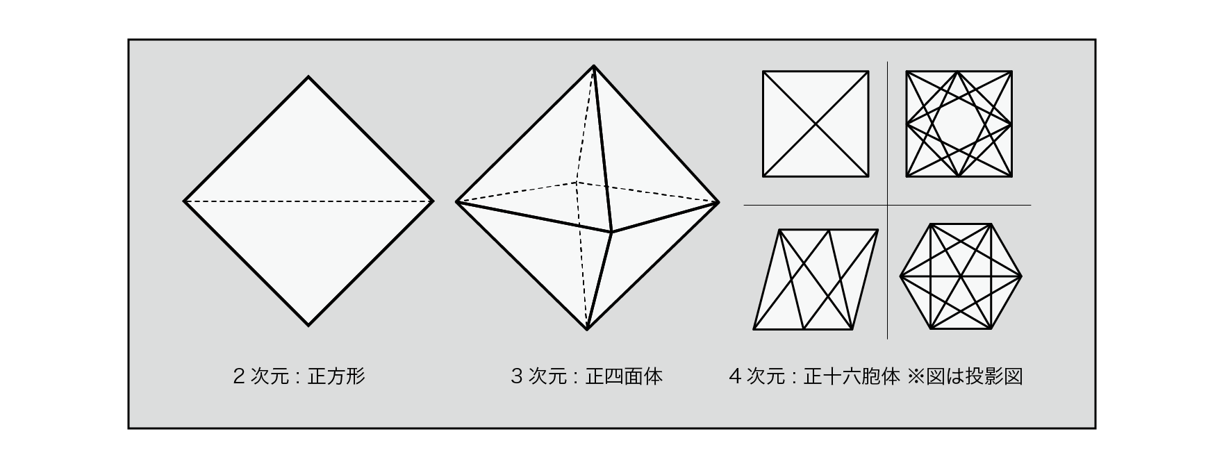
Figure 5.27: Cross-polytope in each dimension
Gradient vector at each dimension, if the two-dimensional square , if a three-dimensional regular octahedral , if four-dimensional (truncated portion) 16-cell of the surface and distributed.
Each dimension and equation are as follows.
2-D: x0 ∈ [−2, 2], y = 1 − |x0|
if y > 0 then x = x0 else x = x0 − sign(x0)

3-D: x0, y0 ∈ [−1, 1], z = 1 − |x0| − |y0|
if z > 0 then x = x0, y = y0
else x = x0 − sign(x0), y = y0 − sign(y0)

4-D: x0, y0, z0 ∈ [−1, 1], w = 1.5 - | x0 | - | y0 | - | z0 |
if w > 0 then x = x0, y = y0, z = z0
else x = x0 − sign(x0), y = y0 − sign(y0), z = z0 − sign(z0)
Most Perlin Noise implementations used gradient vectors of equal magnitude. However, there is a difference in length between the shortest and longest vectors on the surface of the N-dimensional cross-polytope by the factor of \ sqrt {N} . This does not cause strong artifacts, but at higher dimensions the noise pattern becomes less isotropic without explicit normalization of this vector. Normalization is the process of aligning a vector to 1 by dividing the vector by the size of the vector. Assuming that the magnitude of the gradient vector is r , normalization can be achieved by multiplying the gradient vector by the inverse square root of r \ dfrac {1} {\ sqrt {r}} . Here, to improve performance, this inverse square root is approximately calculated using the Taylor expansion. The Taylor expansion is that in an infinitely differentiable function, if x is in the vicinity of a, it can be approximately calculated by the following formula.
\sum ^{\infty }_{n=0}\dfrac {f^{\left( n\right) }\left( a\right) }{n!}\left( x-a\right) ^{n}
Finding the first derivative of \ dfrac {1} {\ sqrt {a}}
\begin{array}{l}
f\left( a\right) =\dfrac {1}{\sqrt {a}}=a^{-\frac{1}{2}}\\
f'\left( a\right) =-\dfrac {1}{2}a^{-\frac{3}{2}}\\
\end{array}
Therefore, the approximate expression in the vicinity of a by Taylor expansion is as follows.
\sum ^{\infty }_{n=0}\dfrac {f^{\left( n\right) }\left( a\right) }{n!}\left( x-a\right) ^{n}
\begin{array}{l}
=a^{-\frac{1}{2}}-\frac{1}{2}a^{-\frac{3}{2}}\left( x-a\right)\\
=\frac{3}{2}a^{-\frac{1}{2}}-\frac{1}{2}a^{-\frac{3}{2}}x\\
\end{array}
Here, if a = 0.7 (I think it is because the length range of the gradient vector is 0.5 to 1.0), 1.79284291400159 --0.85373472095314 * x is obtained.
This is what the implementation looks like.
float3 taylorInvSqrt(float3 r)
{
    return 1.79284291400159 - 0.85373472095314 * r;
}
In the sample project
TheStudyOfProceduralNoise/Scenes/ShaderExampleList
When you open the scene, you can see the implementation result of Simplex Noise . The implemented code is
It is in.
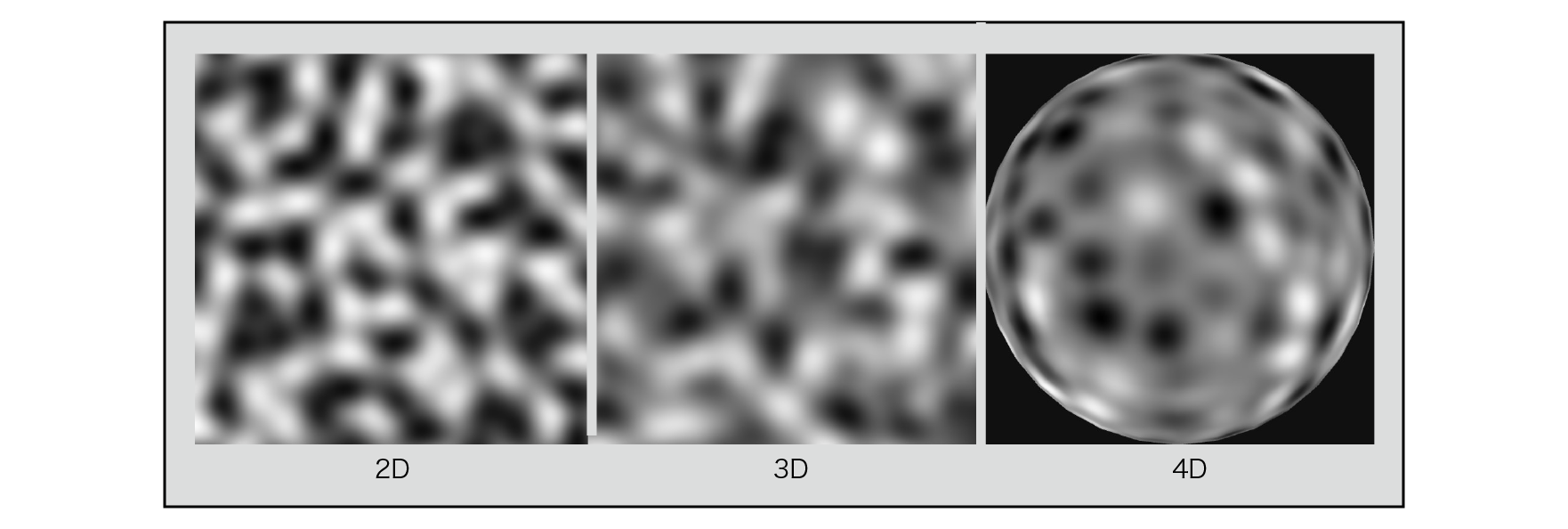
Figure 5.28: Simplex Noise (2D, 3D, 4D) results
Simplex Noise gives a slightly grainier result when compared to Perlin Noise .
We have looked at the algorithms and implementations of typical procedural noise methods in detail, but you can see that there are differences in the characteristics of the noise patterns obtained and the calculation costs. When noise is used in a real-time application, when it becomes high resolution, the calculation is performed for each pixel, so this calculation load cannot be ignored, and what kind of calculation is performed. Should be kept in mind to some extent. Nowadays, many noise functions are built into the development environment from the beginning, but it is important to understand the noise algorithm in order to make full use of it. I couldn't explain its application here, but in graphics generation, the application of noise is extremely diverse and has a great effect. (The next chapter will show one example.) We hope this article provides a foothold for countless applications. Finally, I would like to pay tribute to the wisdom that our predecessors have accumulated and primarily to Ken Perlin's outstanding achievements.